Tutorial
This tutorial works through a real-world example using the New York City Taxi dataset which has been used heavliy around the web (see: Analyzing 1.1 Billion NYC Taxi and Uber Trips, with a Vengeance and A Billion Taxi Rides in Redshift) due to its 1 billion+ record count and scripted process available on github.
It is a great dataset as it has a lot of the attributes of real-world data we want to demonstrate:
- Schema Evolution where fields are added/changed/removed over time or data is normalized as patterns emerge.
- How to reliably apply data typing to an untyped source - in this case Comma-Separated Values format.
- How to build a repeatable and reproducible process which will scale by adding more compute - the small example is ~40 million records and the large 1+ billion records.
- How reusable components can be composed to extract data with data types, apply rules to ensure data quality, enrich the data by executing SQL statements, apply machine learning transformations and load the data to one or more destinations.
Get arc-starter
The easiest way to build an Arc job is by using arc-starter which is an interactive development environment using the Jupyter Notebooks ecosystem. This tutorial assumes you have cloned this repository.
git clone https://github.com/seddonm1/arc-starter.git
cd arc-starter
Get the Data
In the repository there is a directory called tutorial and in that directory there is a directory called data. It already contains subsets of the New York City Taxi dataset stored as gzip archives. The tutorial can be run with these included files.
Alternatively, for a larger dataset, there are two scripts in that directory download_raw_data_large.sh and download_raw_data_small.sh. The small version will download data for approximately 40 million records (6.3GB) and the large will download more than one billion rows of data. Either of these files can be used with this tutorial.
cd tutorial/data
./download_raw_data_small.sh
After that comand runs there should be a directory structure like this the /data directory:
./raw_data_urls_small.txt
./green_tripdata
./green_tripdata/0
./green_tripdata/0/green_tripdata_2013-09.csv
./green_tripdata/0/green_tripdata_2013-08.csv
./green_tripdata/1
./green_tripdata/1/green_tripdata_2015-01.csv
./green_tripdata/2
./green_tripdata/2/green_tripdata_2016-07.csv
./raw_data_urls_large.txt
./central_park_weather
./central_park_weather/0
./central_park_weather/0/central_park_weather.csv
./download_raw_data_large.sh
./download_raw_data_small.sh
./uber_tripdata
./uber_tripdata/0
./uber_tripdata/0/uber-raw-data-apr14.csv
./yellow_tripdata
./yellow_tripdata/0
./yellow_tripdata/0/yellow_tripdata_2009-01.csv
./yellow_tripdata/1
./yellow_tripdata/1/yellow_tripdata_2015-01.csv
./yellow_tripdata/3
./yellow_tripdata/3/yellow_tripdata_2017-01.csv
./yellow_tripdata/2
./yellow_tripdata/2/yellow_tripdata_2016-07.csv
./reference
./reference/cab_type_id.json
./reference/payment_type_id.json
./reference/nyct2010.geojson
./reference/taxi_zones.geojson
./reference/vendor_id.json
Structuring Input Data
One of the key things to notice here is that the download script will create multiple directories for each distinct dataset/table. This is deliberate as each directory will correspond to one version of the schema for that dataset to support Schema Evolution. The directory structure seen above was built based on the rules in this file in the original repository. So for example:
./data/green_tripdata/is the base directory for all data relating to thegreen_tripdatatable../data/green_tripdata/0/is the source directory for all data which meets the first version of the schema. The download script deliberately adds multiple files to this directory to show how the framework can read multiple files per data version../data/green_tripdata/1/is the source directory for all data which meets the second version of the schema which was first seen in the filegreen_tripdata_2015-01.csv. The assumption here is that any file received prior to2015-01should have the same schema as the rest of the files in./data/green_tripdata/0/and so be downloaded to./data/green_tripdata/0/../data/green_tripdata/2/is the source directory for all data which meets the third version of the schema which was first seen in the filegreen_tripdata_2016-07.csv.
At this stage we have not specified what or how to apply a schema we have just physically partitioned the data in to directories that can then be used to find all the files relating to a specific version of a schema.
Starting Jupyter
To start arc-juptyer run the following command. The only option that needs to be configured is the -Xmx4096m to set the memory availble to Spark. This value needs to be less than or equal to the amount of memory allocated to Docker.
docker run \
--name arc-jupyter \
--rm \
-v $(pwd)/tutorial:/home/jovyan/tutorial \
-e JAVA_OPTS="-Xmx4096m" \
-p 4040:4040 \
-p 8888:8888 \
seddonm1/arc-jupyter:0.0.12 \
start-notebook.sh \
--NotebookApp.password='' \
--NotebookApp.token=''
Starting an Arc notebook
From the Juptyter main screen select New then Arc under notebook. We will be building the job in this notebook.
Before we start adding job stages we need to define a variable which allows us to easily change the input file location when we deploy the job across different environments. So, for example, it could be use to switch data paths for local (ETL_CONF_BASE_URL=/home/jovyan/tutorial) vs remote ETL_CONF_BASE_URL=hdfs://datalake/ when moving from development to production.
Paste this into the first sell and execute to set the environment variable.
%env ETL_CONF_BASE_URL=/home/jovyan/tutorial
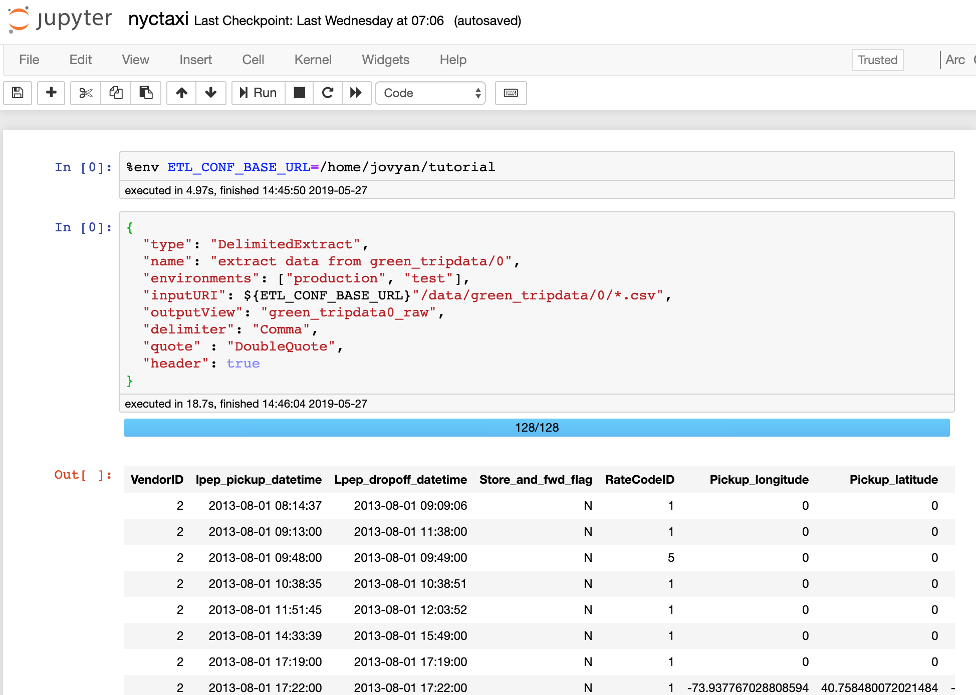
Extracting Data
The first stage we are going to add is a DelimitedExtract stage because the source data is in Comma-Seperated Values format delimited by ‘,’. This stage will instruct Spark to extract the data in all .csv files from the inputURI path and register as a Spark internal view green_tripdata0_raw so the data can be accessed in subsequent job stages.
{
  "type": "DelimitedExtract",
  "name": "extract data from green_tripdata/0",
  "environments": ["production", "test"],
  "inputURI": ${ETL_CONF_BASE_URL}"/data/green_tripdata/0/*",
  "outputView": "green_tripdata0_raw",
  "delimiter": "Comma",
  "quote" : "DoubleQuote",
  "header": true
}
By executing this stage you should be able to see a result set. If you scroll to the very right of the result set you should be able to see two additional columns which is added by Arc to help trace data lineage to assist debugging.
_filename: which records the input file source for all file based imports._index: which records the input file row number for all file based imports.
Typing Data
At this stage we have a stage which will tell Spark where to read one or more .csv files and produce a table that looks like this and has all string typed fields.
| VendorID | lpep_pickup_datetime | Lpep_dropoff_datetime | Store_and_fwd_flag | RateCodeID | Pickup_longitude | Pickup_latitude | Dropoff_longitude | Dropoff_latitude | Passenger_count | Trip_distance | Fare_amount | Extra | MTA_tax | Tip_amount | Tolls_amount | Ehail_fee | Total_amount | Payment_type | Trip_type |
|---|---|---|---|---|---|---|---|---|---|---|---|---|---|---|---|---|---|---|---|
| 2 | 2013-09-01 00:02:00 | 2013-09-01 00:54:51 | N | 1 | -73.952407836914062 | 40.810726165771484 | -73.983940124511719 | 40.676284790039063 | 5 | 14.35 | 50.5 | 0.5 | 0.5 | 10.3 | 0 | null | 61.8 | 1 | null |
| 2 | 2013-09-01 00:02:34 | 2013-09-01 00:20:59 | N | 1 | -73.963020324707031 | 40.711833953857422 | -73.966644287109375 | 40.681690216064453 | 1 | 3.24 | 15 | 0.5 | 0.5 | 0 | 0 | null | 16 | 2 | null |
To make this data more useful for querying (for example doing aggregation by time period) we need to safely apply data typing.
Add a new stage to apply a TypingTransformation to the data extracted in the first stage named green_tripdata0_raw which will parse the data and produce an output dataset called green_tripdata0 with correctly typed data. To do this we have to tell Spark how to parse the text data back into their original data types. To do this transformation we need some way to pass in the description of how to parse the data and that is descriped in the metadata file passed in using the inputURI key and described in the next step.
{
  "type": "TypingTransform",
  "name": "apply green_tripdata/0 data types",
  "environments": ["production", "test"],
  "inputURI": ${ETL_CONF_BASE_URL}"/meta/green_tripdata/0/green_tripdata.json",
  "inputView": "green_tripdata0_raw",
  "outputView": "green_tripdata0"
}
Specifying Data Typing Rules
The metadata format provides the information needed to parse an untyped dataset into a typed dataset. Where a traditional database will fail when a data conversion fails (for example CAST('abc' AS INT)) Spark defaults to returning nulls which makes safely and precisely parsing data using only Spark very difficult.
Metadata Order
This format does not use input field names and will only try to convert data by its column index - meaning that the order of the fields in the metadata file must match the input dataset.
Here is the top of of the tutorial/meta/green_tripdata/0/green_tripdata.json file which provides the detailed metadata of how to convert string values back into their correct data types. The description fields have come from the official data dictionary.
[
  {
    "id": "f457e562-5c7a-4215-a754-ab749509f3fb",
    "name": "vendor_id",
    "description": "A code indicating the TPEP provider that provided the record.",
    "trim": true,
    "nullable": true,
    "primaryKey": false,
    "type": "integer",
    "nullableValues": [
      "",
      "null"
    ]
  },
  {
    "id": "d61934ed-e32e-406b-bd18-8d6b7296a8c0",
    "name": "lpep_pickup_datetime",
    "description": "The date and time when the meter was engaged.",
    "trim": true,
    "nullable": true,
    "primaryKey": false,
    "type": "timestamp",
    "formatters": [
      "uuuu-MM-dd HH:mm:ss"
    ],
    "timezoneId": "America/New_York",
    "nullableValues": [
      "",
      "null"
    ]
  },
  {
    "id": "d61934ed-e32e-406b-bd18-8d6b7296a8c0",
    "name": "lpep_dropoff_datetime",
    "description": "The date and time when the meter was disengaged.",
    "trim": true,
    "nullable": true,
    "primaryKey": false,
    "type": "timestamp",
    "formatters": [
      "uuuu-MM-dd HH:mm:ss"
    ],
    "timezoneId": "America/New_York",
    "nullableValues": [
      "",
      "null"
    ]
  },
  ...
Picking one of the more interesting fields, lpep_pickup_datetime, a timestamp field, we can highlight a few details:
- the
idvalue is a unique identifier for this field (in this case astringformatteduuid). This field can be used to help track changes in the business intent of the field, for example if the field changed name fromlpep_pickup_datetimeto justpickup_datetimein a subsequent schema it is still the same field as the intent has not changed, just the name so the sameidvalue should be retained. - the
formatterskey specifies anarrayrather than a simplestring. This is because real world data often has multiple date/datetime formats used in a single column. By defining anarrayArc will try to apply each of the formats specified in sequence and only fail if none of the formatters can be successfully applied. - a mandatory
timezoneIdmust be specified. This is because if you work with datetime enough you will find that the only way to reliably work with dates and times across systems is to convert them all to Coordinated Universal Time (UTC) so they can be placed as instantaneous point on a universally continuous time-line. - the
nullableValueskey also specifies anarraywhich allows you to specify multiple values which will be converted to a truenullwhen loading. If these values are present and thenullablekey is set totruethen the job will fail with a clear error message. - the description field is saved with the data some formats like when using ORCLoad or ParquetLoad into the underlying metadata and will be restored automatically if those files are re-injested by Spark.
  {
    "id": "d61934ed-e32e-406b-bd18-8d6b7296a8c0",
    "name": "lpep_pickup_datetime",
    "description": "The date and time when the meter was engaged.",
    "trim": true,
    "nullable": true,
    "primaryKey": false,
    "type": "timestamp",
    "formatters": [
      "uuuu-MM-dd HH:mm:ss"
    ],
    "timezoneId": "America/New_York",
    "nullableValues": [
      "",
      "null"
    ]
  },
Decimal vs Float
Because we are dealing with money we are using the decimal type rather than a float. See the documentation for more.
So what happens if this conversion fails?
Data Load Validation
The TypingTransformation silently adds an addition field to each row called _errors which holds an array of data conversion failures - if any exist - so that each row can be parsed and multiple issues collected. If a data conversion issue exists then the field name and a human readable message will be pushed into that array and the value will be set to null for that field:
For example:
+-------------------+-------------------+--------------------------------------------------------------------------------------------------------------------------------------------------------------------------------------------------------------------------------------------------------------------+
|startTime          |endTime            |_errors                                                                                                                                                                                                                                                             |
+-------------------+-------------------+--------------------------------------------------------------------------------------------------------------------------------------------------------------------------------------------------------------------------------------------------------------------+
|2018-09-26 17:17:43|2018-09-27 17:17:43|[]                                                                                                                                                                                                                                                                  |
|2018-09-25 18:25:51|2018-09-26 18:25:51|[]                                                                                                                                                                                                                                                                  |
|null               |2018-03-01 12:16:40|[[startTime, Unable to convert '2018-02-30 01:16:40' to timestamp using formatters ['uuuu-MM-dd HH:mm:ss'] and timezone 'UTC']]                                                                                                                                     |
|null               |null               |[[startTime, Unable to convert '28 February 2018 01:16:40' to timestamp using formatters ['uuuu-MM-dd HH:mm:ss'] and timezone 'UTC'], [endTime, Unable to convert '2018-03-2018 01:16:40' to timestamp using formatters ['uuuu-MM-dd HH:mm:ss'] and timezone 'UTC']]|
+-------------------+-------------------+--------------------------------------------------------------------------------------------------------------------------------------------------------------------------------------------------------------------------------------------------------------------+
If you have specified that the field cannot be null via "nullable": false then the job will fail at this point with an appropriate error message.
If the job has been configured like above with all fields "nullable": true then the TypingTransform stage will complete but we will not be actually asserting that no errors are allowed. To add the ability to stop the job based on whether errors occured we can add a SQLValidate stage:
{
  "type": "SQLValidate",
  "name": "ensure no errors exist after data typing",
  "environments": ["production", "test"],
  "inputURI": ${ETL_CONF_BASE_URL}"/notebooks/0/sqlvalidate_errors.sql",
  "sqlParams": {
      "table_name": "green_tripdata0"
  }
}
When this stage executes it is reading a file contained with the tutorial which contains:
SELECT
  SUM(error) = 0 AS valid
  ,TO_JSON(NAMED_STRUCT('count', COUNT(error), 'errors', SUM(error))) AS message
FROM (
  SELECT
    CASE
      WHEN SIZE(_errors) > 0 THEN 1
      ELSE 0
    END AS error
  FROM ${table_name}
) input_table
The summary of what happens in this SQL statement is:
- sum up the number of rows where the
SIZEof the_errorsarray for each row is greater than 0. If the array is not empty then there must have been at least one error on that row (SIZE(_errors) > 0) - check that that sum of errors
SUM(error) = 0as a predicate so that the first field will returntrueifSUM(error) = 0orfalseifSUM(error) != 0 - as doing a count is visiting all rows anyway we can emit statistics so the output will be a
jsonobject that will be added to the logs. In this case we are logging a row count (COUNT(error)) and a count of rows with at least 1 error (SUM(error)) which will return something like{"count":57270,"errors":0}.
One interesting behaviour is that before the SQL statement is executed the framework will allow you to do parameter replacement. So in the definition for the SQLValidate stage there is an key called sqlParams which allows you to specify named parameters:
"sqlParams": {
    "table_name": "green_tripdata0"
}
In this case before the SQL statement is executed the named parameter ${table_name} will be replaced with green_tripdata0 so it will validate the specified dataset. The benefit of this is that the same SQL statement can be used for any dataset after the TypingTransformation stage to ensure there are no data typing errors and all we have to do is specify a different table_name substitution value.
Data Persistence
A TypingTransformation is a big and computationally expensive operation so if you are going to do multiple operations against that dataset (as we are) set the "persist": true option so that Spark will cache the dataset after applying the types.
Execute It
At this stage we have a job which will apply data types to one or more .csv files and execute a SQLValidate stage to ensure that the data could be converted successfully. The Spark ETL framework is packaged with Docker so that you can run the same job on your local machine or a massive compute cluster without having to think about how to package dependencies. The Docker image contains the dependencies files for connecting to most JDBC, XML, Avro and cloud services.
To export a runable job select File\Download As from the Jupyter menu and select Arc (.json). Once exported that file can be executed like:
docker run \
--rm \
-v $(pwd)/tutorial:/home/jovyan/tutorial \
-e "ETL_CONF_ENV=production" \
-e "ETL_CONF_BASE_URL=/home/jovyan/tutorial" \
-p 4040:4040 \
seddonm1/arc:1.13.3 \
bin/spark-submit \
--master local[*] \
--driver-memory=4G \
--driver-java-options="-XX:+UseG1GC -XX:-UseGCOverheadLimit -XX:+UnlockExperimentalVMOptions -XX:+UseCGroupMemoryLimitForHeap" \
--class au.com.agl.arc.ARC \
/opt/spark/jars/arc.jar \
--etl.config.uri=file:///home/jovyan/tutorial/job/0/nyctaxi.json
Going forward to run a different version of the job just change the /job/0 part to the correct version.
As the job runs you will see json formatted logs generated and printed to screen. These can easily be sent to a log management solution for log aggregation/analysis/alerts. The important thing is that our job ran and we can see our message {"count":57270,"errors":0} formatted as numbers so that it can be easily addressed (event.message.count) and summed/compared day by day for monitoring.
{"event":"exit","duration":1724,"stage":{"sqlParams":{"table_name":"green_tripdata0"},"name":"ensure no errors exist after data typing","type":"SQLValidate","message":{"count":57270,"errors":0}},"level":"INFO","thread_name":"main","class":"etl.validate.SQLValidate$","logger_name":"local-1524100083660","timestamp":"2018-04-19 01:08:14.351+0000","environment":"test"}
{"event":"exit","status":"success","duration":10424,"level":"INFO","thread_name":"main","class":"etl.ETL$","logger_name":"local-1524100083660","timestamp":"2018-04-19 01:08:14.351+0000","environment":"test"}
A snapshot of what we have done so far should be in the repository under tutorial/job/0/nyctaxi.ipynb.
JSON vs HOCON
The config file, whilst looking very similar to a json file is actually a Human-Optimized Config Object Notation (HOCON) file. This file format is a superset of json allowing some very useful extensions like Environment Variable substitution and string interpolation. We primarily use it for Environment Variable injection but all its capabilities described here can be utilised.
Add more data
To continue with the green_tripdata dataset example we can now add the other two dataset versions. This will show the general pattern for adding additional data and dealing with Schema Evolution. You can see here that adding more data is just appending additional stages to the stages array.
{"stages": [
  {
    "type": "DelimitedExtract",
    "name": "extract data from green_tripdata/0",
    "environments": ["production", "test"],
    "inputURI": ${ETL_CONF_BASE_URL}"/data/green_tripdata/0/*",
    "outputView": "green_tripdata0_raw",
    "delimiter": "Comma",
    "quote": "DoubleQuote",
    "header": true
  },
  {
    "type": "TypingTransform",
    "name": "apply green_tripdata/0 data types",
    "environments": ["production", "test"],
    "inputURI": ${ETL_CONF_BASE_URL}"/meta/green_tripdata/0/green_tripdata.json",
    "inputView": "green_tripdata0_raw",
    "outputView": "green_tripdata0"
  },
  {
    "type": "SQLValidate",
    "name": "ensure no errors exist after data typing",
    "environments": ["production", "test"],
    "inputURI": ${ETL_CONF_BASE_URL}"/job/1/sqlvalidate_errors.sql",
    "sqlParams": {
        "table_name": "green_tripdata0"
    }
  },
  {
    "type": "DelimitedExtract",
    "name": "extract data from green_tripdata/1",
    "environments": ["production", "test"],
    "inputURI": ${ETL_CONF_BASE_URL}"/data/green_tripdata/1/*",
    "outputView": "green_tripdata1_raw",
    "delimiter": "Comma",
    "quote": "DoubleQuote",
    "header": true
  },
  {
    "type": "TypingTransform",
    "name": "apply green_tripdata/1 data types",
    "environments": ["production", "test"],
    "inputURI": ${ETL_CONF_BASE_URL}"/meta/green_tripdata/1/green_tripdata.json",
    "inputView": "green_tripdata1_raw",
    "outputView": "green_tripdata1"
  },
  {
    "type": "SQLValidate",
    "name": "ensure no errors exist after data typing",
    "environments": ["production", "test"],
    "inputURI": ${ETL_CONF_BASE_URL}"/job/1/sqlvalidate_errors.sql",
    "sqlParams": {
        "table_name": "green_tripdata1"
    }
  },
  {
    "type": "DelimitedExtract",
    "name": "extract data from green_tripdata/2",
    "environments": ["production", "test"],
    "inputURI": ${ETL_CONF_BASE_URL}"/data/green_tripdata/2/*",
    "outputView": "green_tripdata2_raw",
    "delimiter": "Comma",
    "quote": "DoubleQuote",
    "header": true
  },
  {
    "type": "TypingTransform",
    "name": "apply green_tripdata/2 data types",
    "environments": ["production", "test"],
    "inputURI": ${ETL_CONF_BASE_URL}"/meta/green_tripdata/2/green_tripdata.json",
    "inputView": "green_tripdata2_raw",
    "outputView": "green_tripdata2"
  },
  {
    "type": "SQLValidate",
    "name": "ensure no errors exist after data typing",
    "environments": ["production", "test"],
    "inputURI": ${ETL_CONF_BASE_URL}"/job/1/sqlvalidate_errors.sql",
    "sqlParams": {
        "table_name": "green_tripdata2"
    }
  }
]}
Now we have three typed and validated datasets in memory. How are they merged?
Merging Data
The real complexity with schema evolution comes defining clear rules with how to deal with fields which are added and removed. In the case of green_tripdata the main change over time is the change from giving specific pickup and dropoff co-ordinates (pickup_longitude, pickup_latitude, dropoff_longitude, dropoff_latitude) in the early datasets to only providing more generalised (and much more anonymous) pickup_location_id and dropoff_location_id geographic regions. The easiest way to deal with this is to use a SQLTransform and manually define the rules for each dataset before UNION ALL the data together. See tutorial/job/1/trips.sql:
Executing SQL
The arc-starter Jupyter notebook allows direct execution of SQL for development by executing a Jupyter ‘magic’ called %sql. To execute a statement you can put:
%sql limit=10
SELECT * FROM green_tripdata0
-- first schema 2013-08 to 2014-12
SELECT
  vendor_id
  ,lpep_pickup_datetime AS pickup_datetime
  ,lpep_dropoff_datetime AS dropoff_datetime
  ,store_and_fwd_flag
  ,rate_code_id
  ,pickup_longitude
  ,pickup_latitude
  ,dropoff_longitude
  ,dropoff_latitude
  ,passenger_count
  ,trip_distance
  ,fare_amount
  ,extra
  ,mta_tax
  ,tip_amount
  ,tolls_amount
  ,ehail_fee
  ,NULL AS improvement_surcharge
  ,total_amount
  ,payment_type AS payment_type_id
  ,NULL AS trip_type_id
  ,NULL AS pickup_location_id
  ,NULL AS dropoff_location_id
FROM green_tripdata0

UNION ALL

-- second schema 2015-01 to 2016-06
SELECT
  vendor_id
  ,lpep_pickup_datetime AS pickup_datetime
  ,lpep_dropoff_datetime AS dropoff_datetime
  ,store_and_fwd_flag
  ,rate_code_id
  ,pickup_longitude
  ,pickup_latitude
  ,dropoff_longitude
  ,dropoff_latitude
  ,passenger_count
  ,trip_distance
  ,fare_amount
  ,extra
  ,mta_tax
  ,tip_amount
  ,tolls_amount
  ,ehail_fee
  ,improvement_surcharge
  ,total_amount
  ,payment_type AS payment_type_id
  ,NULL AS trip_type_id
  ,NULL AS pickup_location_id
  ,NULL AS dropoff_location_id
FROM green_tripdata1

UNION ALL

-- third schema 2016-07 +
SELECT
  vendor_id
  ,lpep_pickup_datetime AS pickup_datetime
  ,lpep_dropoff_datetime AS dropoff_datetime
  ,store_and_fwd_flag
  ,rate_code_id
  ,NULL AS pickup_longitude
  ,NULL AS pickup_latitude
  ,NULL AS dropoff_longitude
  ,NULL AS dropoff_latitude
  ,passenger_count
  ,trip_distance
  ,fare_amount
  ,extra
  ,mta_tax
  ,tip_amount
  ,tolls_amount
  ,ehail_fee
  ,improvement_surcharge
  ,total_amount
  ,payment_type AS payment_type_id
  ,NULL AS trip_type_id
  ,pickup_location_id
  ,dropoff_location_id
FROM green_tripdata2
Then we can define a SQLTransform stage to execute the query:
{
  "type": "SQLTransform",
  "name": "merge green_tripdata_* to create a full trips",
  "environments": ["production", "test"],
  "inputURI": ${ETL_CONF_BASE_URL}"/job/1/trips.sql",
  "outputView": "trips",
  "persist": false
}
A snapshot of what we have done so far is tutorial/job/1/nyctaxi.ipynb.
Add the rest of the tables
Go ahead and:
- add the file loading for the
yellow_tripdataanduber_tripdatafiles. There should be 3 stages for each schema load (DelimitedExtract,TypingTransform,SQLValidate) and a total of 8 schemas so 24 stages plus a singleSQLTransformas the final stage to merge the data. - modify the
SQLTransformto include the new datasets. - run the new version of the job. You may need to increase the ram you have allocated to Spark.
A snapshot of what we have done so far is tutorial/job/2/nyctaxi.ipynb.
Dealing with Empty Datasets
So if you executed the same job as the one that is tutorial/job/2/ the previous job should have failed with "messages":["DelimitedExtract has produced 0 columns and no schema has been provided to create an empty dataframe."] as the second Uber directory (data/uber_tripdata/1) is empty (that was deliberately created to demonstrate this functionality). This is the other part of Schema Evolution we are trying to address: a pre-emptive schema.
Sometimes you want to deploy a change to production before the files arrive and either the job fails or does not include that new data once it starts arriving. Arc supports this by allowing you to specify a schema for an empty dataset so that if no data arrives in a target inputURI directory an empty dataset with the correct columns and column types is emited so that all subsequent stages that depend on that dataset execute without failure.
To fix this issue add a schemaURI key which points to the same metadata file used by the subsequent TypingTransform stage:
{
  "type": "DelimitedExtract",
  "name": "extract data from uber_tripdata/1",
  "environments": ["production", "test"],
  "inputURI": ${ETL_CONF_BASE_URL}"/data/uber_tripdata/1/*",
  "schemaURI": ${ETL_CONF_BASE_URL}"/meta/uber_tripdata/1/uber_tripdata.json",
  "outputView": "uber_tripdata1_raw",
  "delimiter": "Comma",
  "quote": "DoubleQuote",
  "header": true
}
Also because we are testing that file for data quality using SQLValidate we need to change the SQL statement to be able to deal with empty datasets by adding a COALESCE to the first return value:
SELECT
  COALESCE(SUM(error) = 0, TRUE) AS valid
  ,TO_JSON(NAMED_STRUCT('count', COUNT(error), 'errors', SUM(error))) AS message
FROM (
  SELECT
    CASE
      WHEN SIZE(_errors) > 0 THEN 1
      ELSE 0
    END AS error
  FROM ${table_name}
) input_table
Run this job and once it completes you should see in the logs: "records":40540347.
A snapshot of what we have done so far is tutorial/job/3/nyctaxi.ipynb.
Reference Data
As the business problem is better understood it is common to see normalization of data. For example, in the yellow_tripdata0 in the early datasets payment_type was a string field which led to values which were variations on the same intent like cash and CASH. In the later datasets the payment_type has been normailized into a dataset which maps the 'cash' type to the value 2. To normalise this data we first need to load a lookup table which is going to define the rules on how to map payment_type to payment_type_id.
So add these tables to be extracted from the included data/reference directory. They are small but we will be using them potentially a lot of times so set "persist": true.
{
  "type": "JSONExtract",
  "name": "load payment_type_id reference table",
  "environments": ["production", "test"],
  "inputURI": ${ETL_CONF_BASE_URL}"/data/reference/payment_type_id.json",
  "outputView": "payment_type_id",
  "persist": true,
  "multiLine": false
}
{
  "type": "JSONExtract",
  "name": "load cab_type_id reference table",
  "environments": ["production", "test"],
  "inputURI": ${ETL_CONF_BASE_URL}"/data/reference/cab_type_id.json",
  "outputView": "cab_type_id",
  "persist": true,
  "multiLine": false
}
{
  "type": "JSONExtract",
  "name": "load vendor_id reference table",
  "environments": ["production", "test"],
  "inputURI": ${ETL_CONF_BASE_URL}"/data/reference/vendor_id.json",
  "outputView": "vendor_id",
  "persist": true,
  "multiLine": false
}
JSON multiLine
In early versions of Spark the only option for json datasets was to use a json format called jsonlines which requires each json object to be on a single line and multiple json objects could appear by having multiple lines of json data. This mode can still be enabled by setting "multiLine": false but the default in Spark ETL is a single json object per file. For reference data, like the data loaded above, we have used a jsonlines file to load multiple records in a single json file.
The main culprit of non-normalized data is the yellow_tripdata0 dataset so let’s add a SQLTransform stage which will do a LEFT JOIN to the new reference data then a SQLValidate stage to check that all of our refrence table lookups were successful (think foreign key integrity). The use of a LEFT JOIN over an INNER JOIN is that we don’t want to filter out data from yellow_tripdata0 that doesn’t have a lookup value.
{
  "type": "SQLTransform",
  "name": "perform lookups for yellow_tripdata0 reference tables",
  "environments": ["production", "test"],
  "inputURI": ${ETL_CONF_BASE_URL}"/job/4/yellow_tripdata0_enrich.sql",
  "outputView": "yellow_tripdata0_enriched",
  "persist": true
}
{
  "type": "SQLValidate",
  "name": "ensure that yellow_tripdata0 reference table lookups were successful",
  "environments": ["production", "test"],
  "inputURI": ${ETL_CONF_BASE_URL}"/job/4/yellow_tripdata0_enrich_validate.sql"
}
Where job/4/yellow_tripdata0_enrich.sql does the LEFT JOINs:
SELECT
  yellow_tripdata0.vendor_name
  ,vendor_id.vendor_id
  ,trip_pickup_datetime AS pickup_datetime
  ,trip_dropoff_datetime AS dropoff_datetime
  ,store_and_fwd_flag
  ,rate_code_id
  ,start_lon AS pickup_longitude
  ,start_lat AS pickup_latitude
  ,end_lon AS dropoff_longitude
  ,end_lat AS dropoff_latitude
  ,passenger_count
  ,trip_distance
  ,fare_amt AS fare_amount
  ,surcharge AS extra
  ,mta_tax
  ,tip_amount
  ,tolls_amount
  ,NULL AS ehail_fee
  ,NULL AS improvement_surcharge
  ,total_amount
  ,LOWER(yellow_tripdata0.payment_type) AS payment_type
  ,payment_type_id.payment_type_id
  ,NULL AS trip_type
  ,NULL AS pickup_nyct2010_gid
  ,NULL AS dropoff_nyct2010_gid
  ,NULL AS pickup_location_id
  ,NULL AS dropoff_location_id
FROM yellow_tripdata0
LEFT JOIN vendor_id ON yellow_tripdata0.vendor_name = vendor_id.vendor
LEFT JOIN payment_type_id ON LOWER(yellow_tripdata0.payment_type) = payment_type_id.payment_type
… and then SQLValidate verifies that there are no missing values. This query will also collect up the distinct list of missing values so they can be logged and added manually added to the lookup table if required.
SELECT
  SUM(null_vendor_id) = 0 AND SUM(null_payment_type_id) = 0 AS valid
  ,TO_JSON(
    NAMED_STRUCT(
      'null_vendor_id'
      ,SUM(null_vendor_id)
      ,'null_vendor_name'
      ,COLLECT_LIST(DISTINCT null_vendor_name)
      ,'null_payment_type_id'
      ,SUM(null_payment_type_id)
      ,'null_payment_type'
      ,COLLECT_LIST(DISTINCT null_payment_type)
    )
  ) AS message
FROM (
  SELECT
    CASE WHEN vendor_id IS NULL THEN 1 ELSE 0 END AS null_vendor_id
    ,CASE WHEN vendor_id IS NULL THEN vendor_name ELSE NULL END AS null_vendor_name
    ,CASE WHEN payment_type_id IS NULL THEN 1 ELSE 0 END AS null_payment_type_id
    ,CASE WHEN payment_type_id IS NULL THEN payment_type ELSE NULL END AS null_payment_type
  FROM yellow_tripdata0_enriched
) valid
Which will succeed with "message":{"null_payment_type":[],"null_payment_type_id":0,"null_vendor_id":0,"null_vendor_name":[]}.
So now we have a job which will merge all the *tripdata datasets into a single master trips dataset.
A snapshot of what we have done so far is tutorial/job/4/nyctaxi.ipynb.
Saving Data
The final step is to do something with the merged data. This could be any of the Load stages but for our use case we will do a ParquetLoad. Apache Parquet is a great because:
- it is a columnar data format which means that when it is read by subsequent Spark jobs you can only read the columns that are required vastly reducing the amount of data moved across a network and that has to be processed.
- it retains full data types and metadata so that you don’t have to keep converting text to correctly typed data
- it supports data partitioning and pushdown which also reduces the amount of data required to be processed
Here is the stage we will add which writes the trips dataset to a parquet file on disk. It will also be partitioned by vendor_id so that if you were doing analysis on only one of the vendors then Spark could easily read only that data and ignore the other vendors.
{
    "type": "ParquetLoad",
    "name": "write trips back to filesystem",
    "environments": ["production", "test"],
    "inputView": "trips",
    "outputURI": ${ETL_CONF_BASE_URL}"/data/output/trips.parquet",
    "numPartitions": 100,
    "partitionBy": [
        "vendor_id"
    ]
}
A snapshot of what we have done so far is tutorial/job/5/nyctaxi.ipynb.
Applying Machine Learning
There are multiple ways to execute Machine Learning using Arc:
- HTTPTransform allows calling an externally hosted model via HTTP.
- TensorFlowServingTransform allows calling a model hosted in a TensorFlow Serving container.
- MLTransform allows executing pretrained Spark ML model.
Assuming you have executed the job up to stage 5 we will use the trips.parquet file to train a new Spark ML model to attempt to predict the fare based on other input values. It is suggested to use a SQL statement to perform feature creation as even though SQL is clumsy compared with the brevity of Python Pandas it is automatically parallelizable by Spark and so can easily perform on 1 or n CPU cores without modification. It is also very easy to find people who can understand the logic:
-- enrich the data by:
-- - filtering bad data
-- - one-hot encode hour component of pickup_datetime
-- - one-hot encode dayofweek component of pickup_datetime
-- - calculate duration in seconds
-- - adding flag to indicate whether pickup/dropoff within jfk airport bounding box
SELECT
  *
  ,CAST(HOUR(pickup_datetime) = 0 AS INT) AS pickup_hour_0
  ,CAST(HOUR(pickup_datetime) = 1 AS INT) AS pickup_hour_1
  ,CAST(HOUR(pickup_datetime) = 2 AS INT) AS pickup_hour_2
  ,CAST(HOUR(pickup_datetime) = 3 AS INT) AS pickup_hour_3
  ,CAST(HOUR(pickup_datetime) = 4 AS INT) AS pickup_hour_4
  ,CAST(HOUR(pickup_datetime) = 5 AS INT) AS pickup_hour_5
  ,CAST(HOUR(pickup_datetime) = 6 AS INT) AS pickup_hour_6
  ,CAST(HOUR(pickup_datetime) = 7 AS INT) AS pickup_hour_7
  ,CAST(HOUR(pickup_datetime) = 8 AS INT) AS pickup_hour_8
  ,CAST(HOUR(pickup_datetime) = 9 AS INT) AS pickup_hour_9
  ,CAST(HOUR(pickup_datetime) = 10 AS INT) AS pickup_hour_10
  ,CAST(HOUR(pickup_datetime) = 11 AS INT) AS pickup_hour_11
  ,CAST(HOUR(pickup_datetime) = 12 AS INT) AS pickup_hour_12
  ,CAST(HOUR(pickup_datetime) = 13 AS INT) AS pickup_hour_13
  ,CAST(HOUR(pickup_datetime) = 14 AS INT) AS pickup_hour_14
  ,CAST(HOUR(pickup_datetime) = 15 AS INT) AS pickup_hour_15
  ,CAST(HOUR(pickup_datetime) = 16 AS INT) AS pickup_hour_16
  ,CAST(HOUR(pickup_datetime) = 17 AS INT) AS pickup_hour_17
  ,CAST(HOUR(pickup_datetime) = 18 AS INT) AS pickup_hour_18
  ,CAST(HOUR(pickup_datetime) = 19 AS INT) AS pickup_hour_19
  ,CAST(HOUR(pickup_datetime) = 20 AS INT) AS pickup_hour_20
  ,CAST(HOUR(pickup_datetime) = 21 AS INT) AS pickup_hour_21
  ,CAST(HOUR(pickup_datetime) = 22 AS INT) AS pickup_hour_22
  ,CAST(HOUR(pickup_datetime) = 23 AS INT) AS pickup_hour_23
  ,CAST(DAYOFWEEK(pickup_datetime) = 0 AS INT) AS pickup_dayofweek_0
  ,CAST(DAYOFWEEK(pickup_datetime) = 1 AS INT) AS pickup_dayofweek_1
  ,CAST(DAYOFWEEK(pickup_datetime) = 2 AS INT) AS pickup_dayofweek_2
  ,CAST(DAYOFWEEK(pickup_datetime) = 3 AS INT) AS pickup_dayofweek_3
  ,CAST(DAYOFWEEK(pickup_datetime) = 4 AS INT) AS pickup_dayofweek_4
  ,CAST(DAYOFWEEK(pickup_datetime) = 5 AS INT) AS pickup_dayofweek_5
  ,CAST(DAYOFWEEK(pickup_datetime) = 6 AS INT) AS pickup_dayofweek_6
  ,UNIX_TIMESTAMP(dropoff_datetime) - UNIX_TIMESTAMP(pickup_datetime) AS duration
  ,CASE
      WHEN
          (pickup_latitude < 40.651381
          AND pickup_latitude > 40.640668
          AND pickup_longitude < -73.776283
          AND pickup_longitude > -73.794694)
          OR
          (dropoff_latitude < 40.651381
          AND dropoff_latitude > 40.640668
          AND dropoff_longitude < -73.776283
          AND dropoff_longitude > -73.794694)
      THEN 1
      ELSE 0
  END AS jfk
FROM trips
WHERE trip_distance > 0
AND pickup_longitude IS NOT NULL
AND pickup_latitude IS NOT NULL
AND dropoff_longitude IS NOT NULL
AND dropoff_latitude IS NOT NULL
To execute the training load the /job/6/New York City Taxi Fare Prediction SparkML.ipynb notebook. It is commented and will describe the process to execute the SQL above to prepare the training dataset and train a model.
Once done the model can be executed in the notebook:
{
  "type": "SQLTransform",
  "name": "merge green_tripdata_* to create a full trips",
  "environments": ["production", "test"],
  "inputURI": ${ETL_CONF_BASE_URL}"/job/6/trips_enriched.sql",
  "outputView": "trips_enriched",
  "persist": false
},
{
  "type": "MLTransform",
  "name": "apply machine learning prediction model",
  "environments": [
    "production",
    "test"
  ],
  "inputURI": ${ETL_CONF_BASE_URL}"/job/6/trips_enriched.model",
  "inputView": "trips_enriched",
  "outputView": "trips_scored"
}
You can now Load the output dataset into a target like parquet or JDBCLoad into a caching database for serving.
A snapshot of what we have done so far is tutorial/job/6/nyctaxi.ipynb.